Flow Around a Stationary Cylinder

MODULE

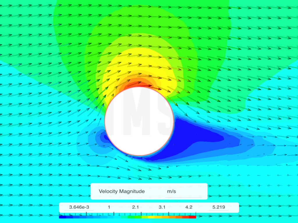
Figure: Simscale Post-Processing of Flow around the Stationary Cylinder

AIM

To quantify the drag coefficient at various Reynolds numbers in the analysis of fluid flow over a stationary cylinder, aiming to comprehend the impact of Reynolds number on drag forces

QUICK PEEK INTO THE TEXTBOOK

Review the TEXTBOOK to refresh your understanding of basic concepts before advancing to more complex material.

FLOW ANALYSIS USING SIMSCALE

COMPLETE TUTORIAL

CLICK TO VIEW THE FINISHED PROJECT

CLICK TO VIEW THE FINISHED PROJECT RESULTS

SimScale Tutorial: Flow around a Stationary Cylinder

This tutorial aims to investigate the pressure drop and visualize the velocity profile in turbulent flow through a pipe.

VIEW THE FINISHED PROJECT

Geometry & Analysis Type

Fluid: Air
Diameter = 0.4 m
Analysis Type: Incompressible steady-state analysis.
Turbulence Model: Laminar flow
Formulae Used:
- edit

1. Prepare the CAD Model and Select the Analysis Type

1.1. Open a ‘New Project’ & import the CAD model

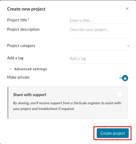
Click open the new project, and fill the details as following dialogue box appears.

Once details are entered, Click ‘Create Project‘.

Click + next to GEOMETRIES, and import the CAD model

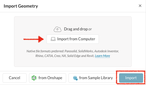
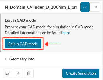
Once imported, click the geometry, and click ‘Edit with CAD mode‘.

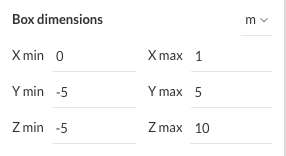
In the CAD mode, select CREATE > External, and enter the following dimensions, for creating the external flow volume. It will get saved as the ‘Flow Region’
NOTE: The external flow volume is more than 5-10 times bigger than the geometry itself.

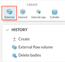
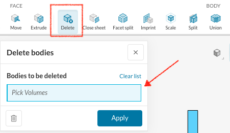
Once the external flow volume has been created, Select DELETE from the options under BODY, and choose the geometry as the volume, and press APPLY.
NOTE: The external flow volume is more than 5-10 times bigger than the geometry itself.

1.2. Create Simulation

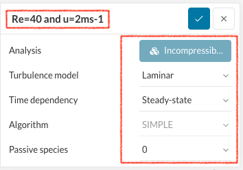
Select ‘Incompressible’ and click Create Simulation and rename it.
Once the Simulation has been created, you can rename it, and choose ‘Laminar‘ to be the Turbulence model and edit the other characteristics as shown here.

2. Assigning the Material and Boundary Conditions

2.1 Define a Material

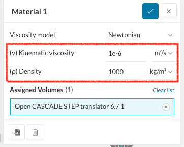
Select any material by clicking ‘+’ next to ‘Material’, and edit its Material Name, and other characteristic features as given.

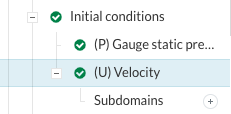
2.2 Define the Initial Conditions

Set the Initial Conditions, namely
- (P) Gauge static pressure = 0 Pa
- (U) Velocity(Global) = 0 m/s

2.2 Define Boundary Conditions

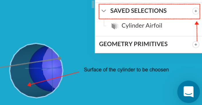
Select + near SAVED SELECTIONS that appears on the right hand side of the workspace.
Choose all the sides of the cylinder, and click APPLY, and save it in a name like ‘Cylinder Airfoil’.
You can now simply select the entire airfoil by selection the SAVED SELECTION without having to choose its faces individually.

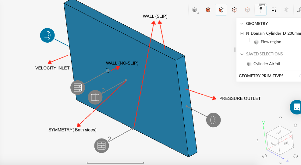
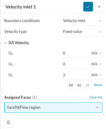
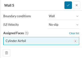
Figure: Boundary Conditions for the Pipe

To set up the ‘Boundary Conditions’, enter the values as given in the snippets, and select the corresponding faces of the geometry.
Set the boundary conditions as given in the following snippets.

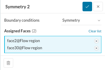
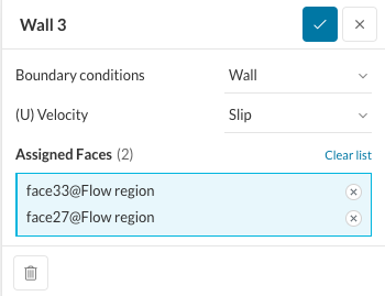
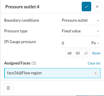
Figure: Pressure Outlet Boundary Condition

2.3. Simulation Control & Result Control

Set the ‘Numerics’ & ‘Simulation Control‘ as given in the ‘FINISHED PROJECT’.
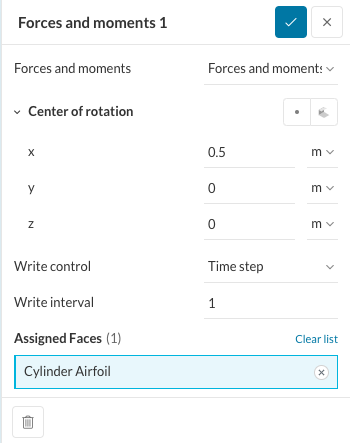
To calculate the ‘Forces and Moments’, enter the values as given in the snippets, and select the Cylindrical Airfoil from the SAVED SELECTION.

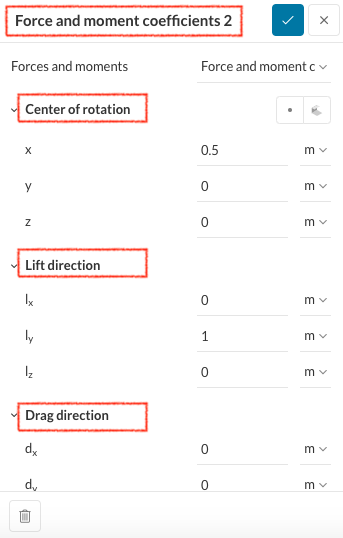
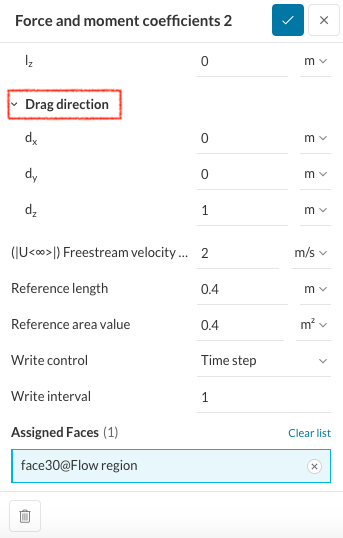
To calculate the ‘Force and Moment Co-efficients’, enter the values as given in the snippets below, and select the Cylindrical Airfoil from the SAVED SELECTION.

3. Mesh

Below the Mesh Settings, Click ‘+’ next to Geometry Primitives, and create the following geometry primitives, which would be used in creating the region refinements in the next step for meshing.

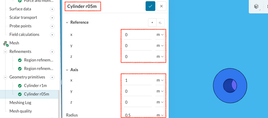
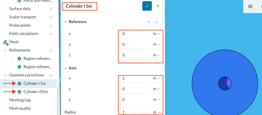
Geometry Primitive Cylinder 1 Creation Set Up

Click on Mesh, and Click ‘+’ next to Refinement, and add the following region refinement for the cylinder.

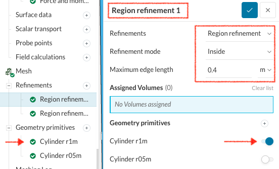
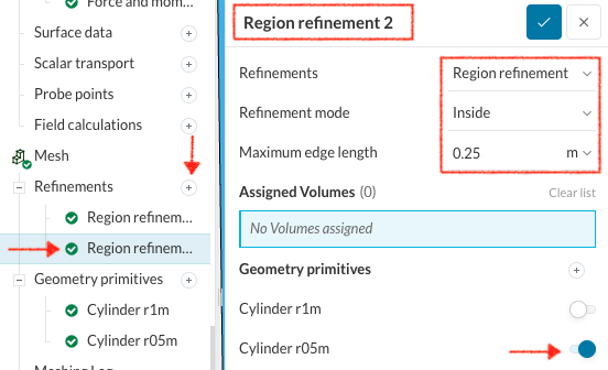
Now after creating the geometry primitives, and adding the suitable region refinements for creating fine mesh, let’s set up the mesh characteristics.

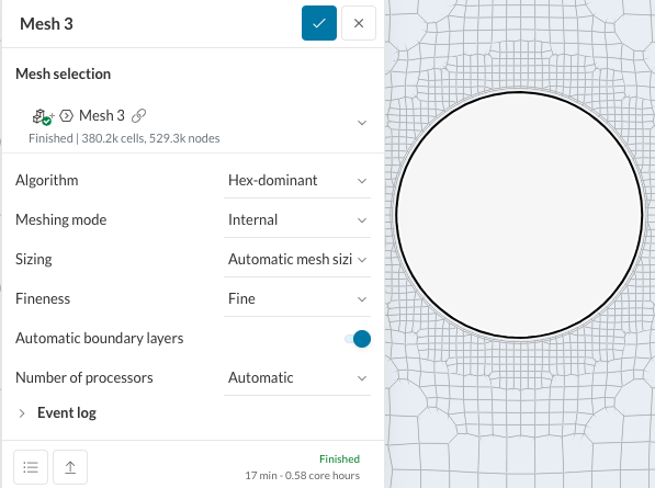
Click on Mesh, and make changes to the Mesh Settings.
Following the above, Click Generate to generate Mesh, and wait for the mesh to get generated.
NOTE: Check the Event Log below the dialogue box once the mesh is generated to check for the mesh quality before proceeding. If the mesh is not correctly generated, Simulation Run in the next stage can get terminated prematurely.

4. Simulation

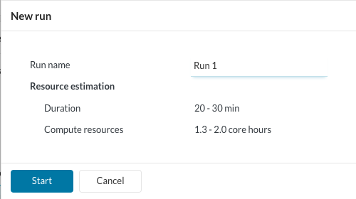
Click ‘+’ next to ‘Simulation Runs‘, and ‘Run‘.

5. Post-Processing

Once the simulation is ‘Complete‘, you can access the post-processing environment by clicking on ‘Solution Fields’ or ‘Post-process results’.

CONTENTS