Overview
This chapter delves into the characteristics of laminar flow within a circular tube, also known as Hagen Poiseuille flow, as well as turbulent flow through the same pipe under varied flow conditions. Unlike drag-induced flow, such as Couette Flow, this type of flow is driven by pressure in a long duct, typically a pipe.
The primary objective of this module is to equip students with a comprehensive understanding of the intricate principles governing fluid flow within a pipe. The focus is on elucidating the concepts of pressure drop in both laminar and turbulent pipe flows, alongside the corresponding velocity profile for fully developed flow. Through the establishment of a predetermined velocity for flow within the pipe, learners will develop the capability to compute pressure drop and visualize it via a series of simulations.
To achieve this objective, two distinct flow scenarios were selected: laminar flow and turbulent flow. The CAD models of these pipes were meticulously designed using SolidWorks, followed by simulations carried out via SimScale.
To ensure the accuracy of the simulation results, extensive comparisons were made with theoretical calculations utilizing conventional formulas for pressure drop computation and visualization of the velocity profile. Additionally, internal consistency checks were conducted by comparing results from different simulation runs, thereby bolstering confidence in the obtained outcomes.
Geometry and Flow Assumptions
The assumptions for this flow problem are as follows:
(i) The flow is laminar and involves an incompressible Newtonian fluid with a given kinematic viscosity.
(ii) The flow is induced by a constant positive pressure difference or pressure drop Δp.
(iii) The flow occurs in a pipe of length L and radius R, where R is much smaller than L.
(iv) The pipe has a circular cross-section normal to its axis, resembling a right circular cylindrical duct.
(v) Over long distances along the pipe, the velocity becomes purely axial and varies solely with the lateral coordinates.
(vi) The flow is considered fully developed, meaning that the velocity components in the radial and circumferential directions are zero, and the axial velocity only varies with the radial coordinate.
Geometry
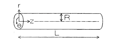
Poiseuille Flow Geometry[19]
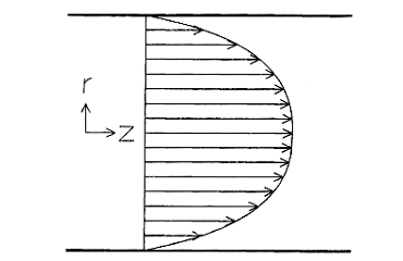
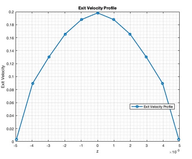
Axial Velocity Profile[19]
The analysis of Poiseuille flow is conducted using cylindrical polar coordinates (r, θ, z), with the origin located on the centerline of the pipe entrance and the z-direction aligned with the centerline. Symmetry in Poiseuille flow implies that the flow is swirl-free and axisymmetric. Consequently, the only non-zero velocity components are the radial component (ur) and the axial component (uz), with the angular component (uθ) being zero. Furthermore, ur and uz are independent of θ, as well as the pressure (p).
Given the elongated nature of the pipe, Poiseuille flow is fully developed, signifying that the velocity u remains constant along the axial position (z) except near the entrance (z = 0) and exit (z = L) of the pipe. Consequently, the radial velocity component (ur) is zero.
Impact of Reynolds Number
Reynolds number characterizes the flow itself, rather than the fluid passing through it. It depends on the flow velocity and a characteristic length, while fluid properties such as viscosity and density play a vital role. This dimensionless quantity gauges the turbulence within a flow by comparing diffusive and advective momentum transport time scales.
Altering the Reynolds number involves adjusting the balance between diffusive and advective momentum transfer. Using a more viscous fluid enhances diffusive momentum transport, thus reducing the Reynolds number. Conversely, increasing flow velocity boosts advective momentum transport, elevating the Reynolds number.
Laminar flow occurs at low Reynolds numbers (below 2300), where resistance is independent of pipe wall roughness. At around 2300, the flow condition becomes critical, exhibit- ing characteristics of both laminar and turbulent flow. Above 2300, turbulent flow dominates at Reynolds numbers. The Reynolds number at which the flow starts transitioning from laminar to turbulent flow, is called the critical Reynolds number (Recritical)
Impact of Internal Roughness and Viscosity on Velocity Profile
Influence of Internal Roughness
The velocity profile within a pipe is significantly influenced by the internal roughness of its surface. When fluid flows through a pipe with smooth walls, like glass or polyethylene, the velocity profile remains relatively uniform. However, in pipes with rougher surfaces such as concrete or steel, the velocity profile becomes distorted. This distortion arises due to the formation of eddy currents within the fluid caused by the irregularities on the pipe’s inner surface. These eddy currents disrupt the smooth flow of the fluid, leading to variations in velocity across the pipe’s cross-section. As a result, fluid near the pipe wall tends to flow more slowly compared to the fluid in the center of the pipe.
Effect of Viscosity
Viscosity also plays a crucial role in shaping the velocity profile within a pipe. In fluids with high viscosity, such as thick oils or syrups, the flow tends to be laminar. In laminar flow, the layers of fluid slide smoothly over each other, resulting in a parabolic velocity profile. The fluid near the pipe wall moves more slowly than the fluid in the center, creating a velocity gradient across the pipe’s cross-section. This gradient is more pronounced in viscous fluids due to their resistance to flow, resulting in a more significant difference in velocity between the layers.
Conversely, in fluids with low viscosity, such as water or air, turbulence may occur, especially at higher flow rates or rougher pipe surfaces. Turbulent flow disrupts the orderly motion of fluid layers, causing mixing and fluctuations in velocity throughout the cross-section of the pipe. As a result, the velocity profile in turbulent flow becomes flatter compared to laminar flow, with less pronounced variations in velocity between the layers.
Overall, both internal roughness and viscosity significantly affect the velocity profile within a pipe, with smoother surfaces and higher viscosity favoring laminar flow and a more predictable velocity distribution, while rougher surfaces and lower viscosity may lead to turbulent flow and greater variability in velocity.
Understanding Friction Factor and Pressure Drop
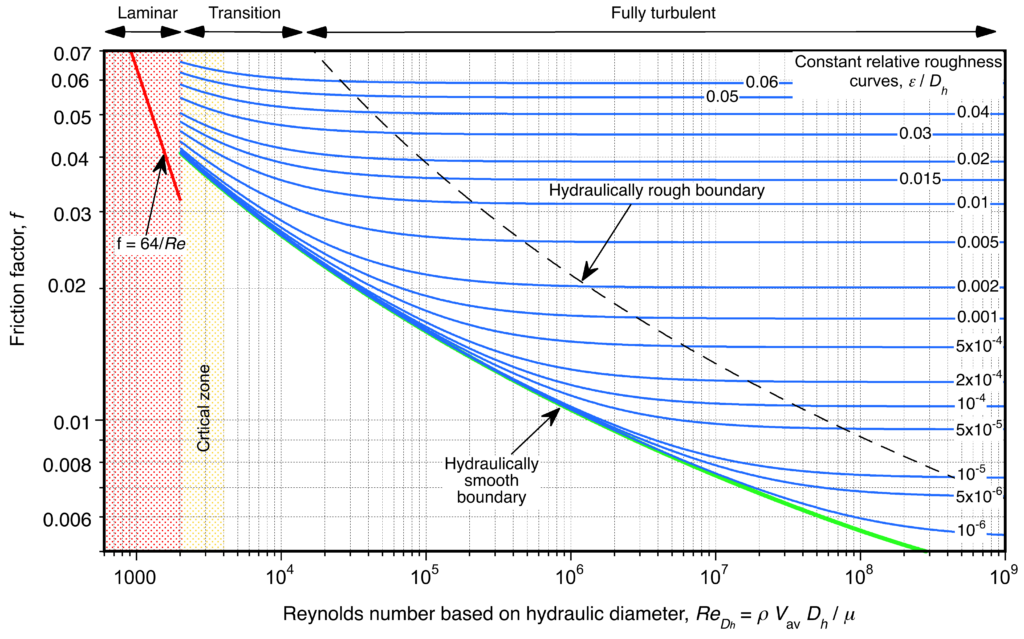
In the entrance region of a pipe, fluid acceleration or deceleration leads to a balance between pressure, viscous, and inertia forces. The friction factor (or Darcy Friction factor) quantifies the dimensionless pressure drop for internal flows. Eddy currents within the flow, relative roughness of the pipe, and Reynolds number together determine the friction factor, i.e., the ratio of internal roughness of the pipe to its diameter. While large diameter pipes mitigate the effect of eddy currents, smaller ones are significantly influenced by internal roughness, which can be plotted using Moody’s chart.
In Laminar flow:
To calculate the friction factor for laminar flow, one can use the formula:
( f =64/Re )
where Re is the Reynolds number. The pressure drop (∆P) for laminar flow can be calculated as:
Δ𝑃 = (128/𝜋)(𝜇𝐿/𝐷4)𝑄
In Turbulent flow :
For turbulent flow, the relative roughness must be found, and then Moody’s diagram can be used to find the friction factor (f). The pressure drop (∆P) for turbulent flow is calculated as:
Δ𝑃 = 𝑓 (𝜌 𝑢2 𝑙2/𝑑)
Validation Results
Here’s a comparison of the simulation results with what’s in the literature, based on the flow simulation conditions given in the tutorials. This helps validate our findings!
NOTE: Refer to the tutorial to view the details of the simulation set-up.
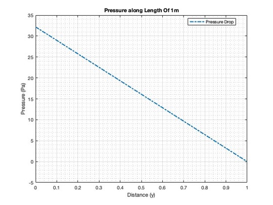
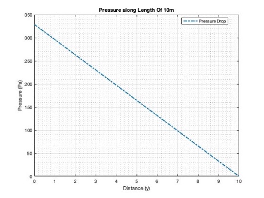
LAMINAR FLOW
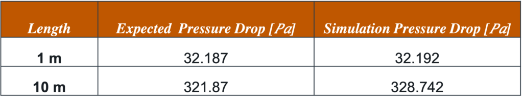
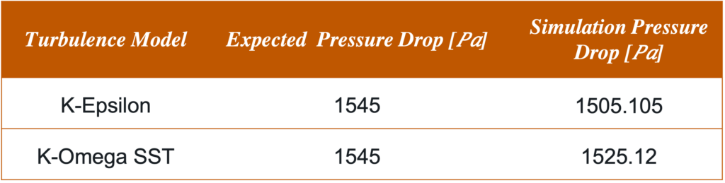
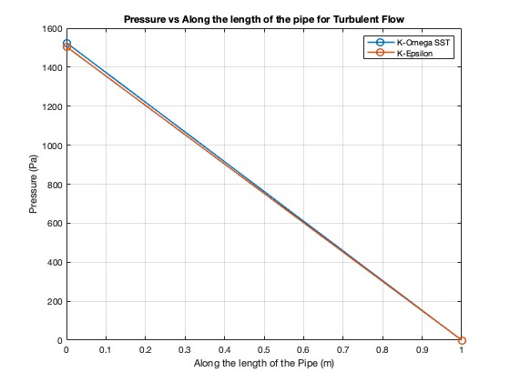
TURBULENT FLOW
Feel free to give plotting the velocity profile for turbulent flow a shot, just like it is shown in the tutorials!
REFERENCES
[17] Richardson, S. M., 2008, “POISEUILLE FLOW,” Begellhouse eBooks.
[20] 2022, “Internal Fluid Flows,” INTRODUCTION TO AEROSPACE FLIGHT VEHICLES, Embry Riddle Aeronautical University.