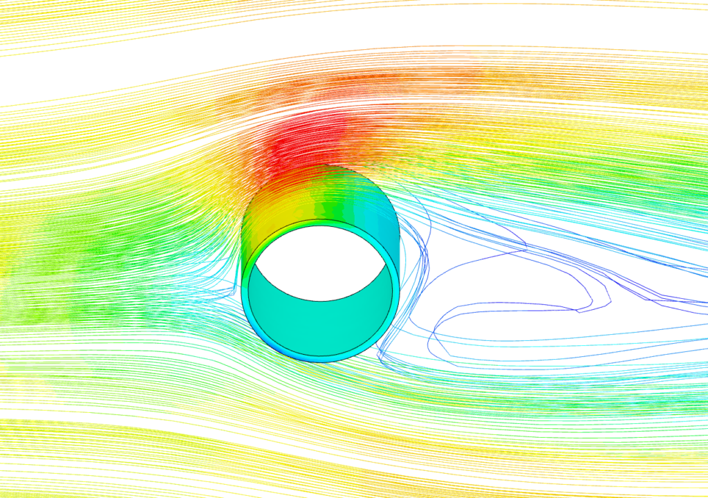
Flow Around a Spinning Cylinder

MODULE

Figure: Simscale Post-Processing of Flow around the Spinning Cylinder

AIM

To quantify the lift coefficient at various Reynolds numbers in the analysis of fluid flow over a Spinning Cylinder, aiming to comprehend the impact of Reynolds number on lift forces

QUICK PEEK INTO THE TEXTBOOK

Review the TEXTBOOK to refresh your understanding of basic concepts before advancing to more complex material.

SimScale Tutorial: Flow around a Spinning Cylinder

This tutorial aims to explore the lift coefficient across various Reynolds numbers when analyzing fluid flow over a spinning cylinder. Our goal is to gain a deeper understanding of how Reynolds number influences lift forces.

VIEW THE FINISHED PROJECT

GET STARTED WITH YOUR OWN PROJECT

FLOW SIMULATION SETUP

Dimensions

Diameter = 0.5642 m

Analysis Type

Incompressible steady-state analysis.

Turbulence Model

k-Omega SST

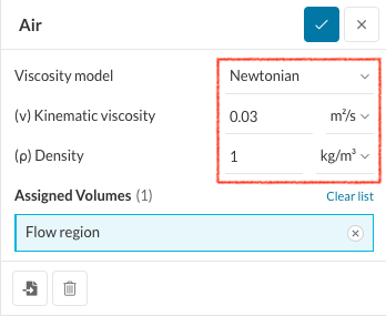
Fluid : Air

Mesh Type

Algorithm – Standard
Sizing – Fine Automated

Initial Conditions

Viscosity Model – Newtonian
(𝜈) Kinematic viscosity = 0.03 𝑚²/s
Rotational Velocity = 1 rad/s
Density = 1 kg/m³

Let’s now delve into the SimScale process one step at a time for this particular problem.

Just a heads-up: The ideal way to begin is by creating a ‘New Project’ and then importing the CAD model. However, we’ve already taken care of the steps for you, including importing the CAD model. You can get started right away with the ‘Creation of Flow Domain‘ step.

Prepare the CAD Model and Select the Analysis Type

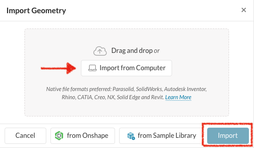
Open a ‘New Project’ & import the CAD model

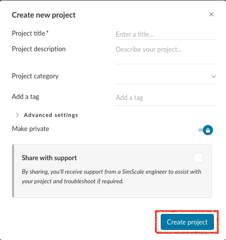
Click open the new project, and fill the details as following dialogue box appears.

Once details are entered, Click ‘Create Project‘.

Click + next to GEOMETRIES, and import the CAD model

Creation of Flow Domain

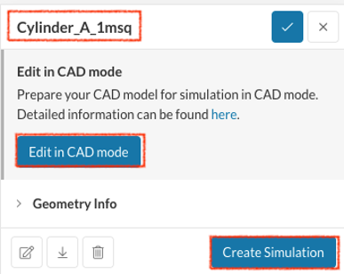
Once imported, click the geometry, and click ‘Edit with CAD mode‘.

NOTE: This issue is a unique instance that pertains to managing rotating zones.

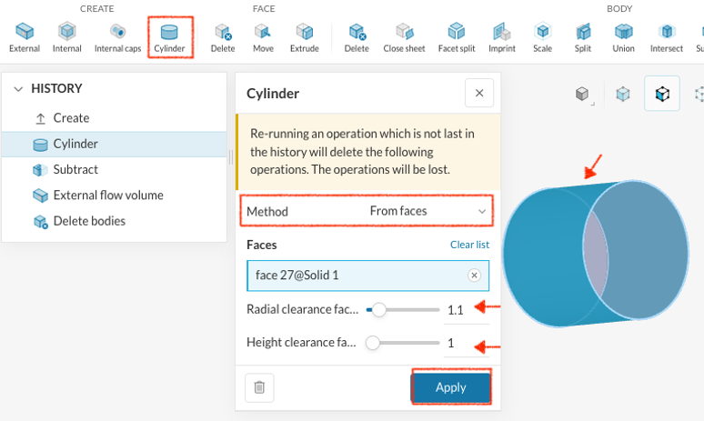
In CAD mode, the Cylinder operation facilitates the generation of cylindrical volumes suitable for simulation domains featuring rotating areas.

Select Cylinder from various options under CREATE.
Select the ‘From faces’ method for cylinder creation.
Choose the specific faces that the cylinder should encompass.
Generate a cylinder using the chosen faces.
Apply a Clearance factor to slightly exceed the designated faces, typically 1.1 for simulations involving rotating machinery.

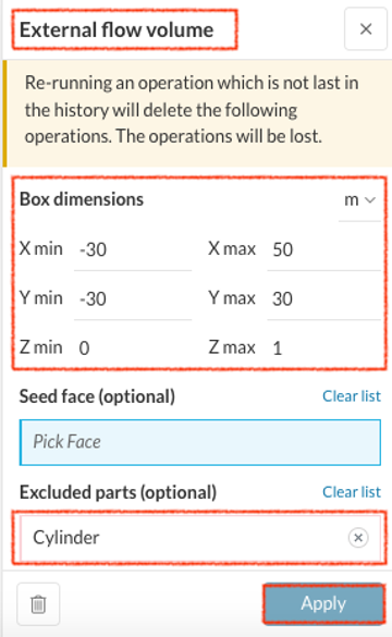
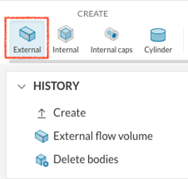
To establish the flow region, navigate to CAD mode and select CREATE > External.
Input the specified dimensions to generate the external flow volume, which will be automatically saved as the ‘Flow Region’.

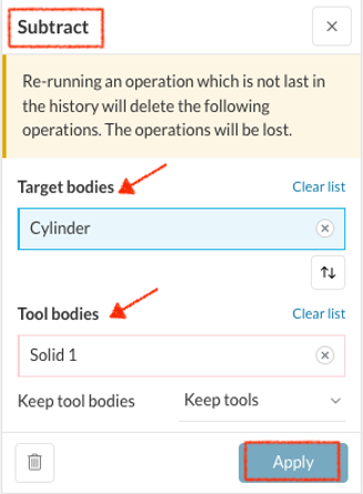
To delete the excess region from the cylinder created, let’s perform the SUBTRACT operation.
Choose the Subtract option.
Select the given target bodies and tool bodies.
Perform the operation by clicking Apply.

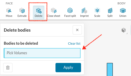
Once the external flow volume has been created, Select DELETE from the options under BODY, and choose the geometry as the volume, and press APPLY.

Create Simulation

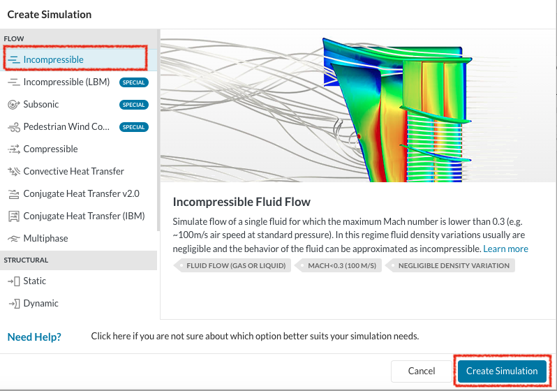
Select ‘Incompressible’ and click Create Simulation
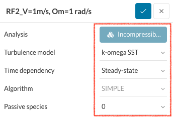
Once the Simulation has been created, you can rename it and edit the characteristics as shown here.

Assigning the Material and Boundary Conditions

Define a Material

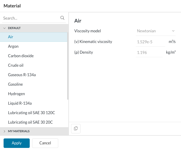
Select any material by clicking ‘+’ next to ‘Material’, and edit its Material Name, and other characteristic features as given.

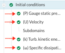
Define the Initial Conditions

Set the Initial Conditions, namely
- (P) Gauge static pressure = 0 Pa
- (U) Velocity(Global) = 0 m/s
- (k) Turb Kinetic Energy = 3.84e-3 m²/s²
- (w) Specific Dissipation Rate = 88.53 1/s

Define Boundary Conditions

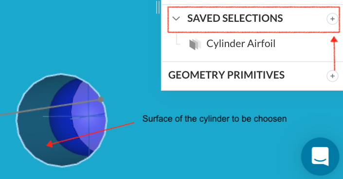
Select + near SAVED SELECTIONS that appears on the right hand side of the workspace.
Choose all the sides of the cylinder, and click APPLY, and save it in a name like ‘Cylinder Airfoil’.
You can now simply select the entire airfoil by selection the SAVED SELECTION without having to choose its faces individually.

To configure the ‘Boundary Conditions‘, input the specified values provided in the snippets and designate the respective faces of the geometry.

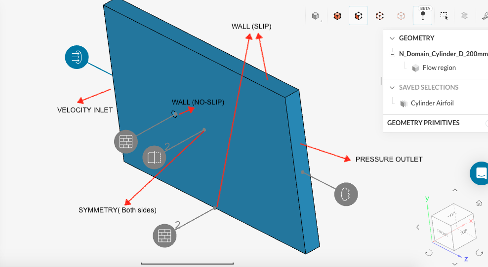
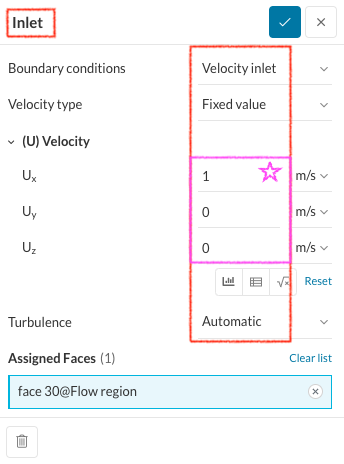
Figure: Boundary Conditions for the Pipe

Set the Inlet boundary condition.

At the conclusion of this tutorial, you will find a table presenting the velocity component sets for various cases. Make sure to follow the tutorial for each specific case.

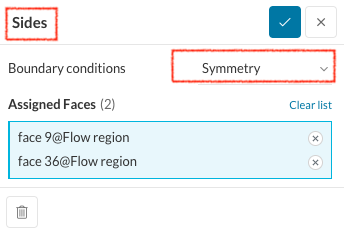
Set the Symmetry boundary condition.

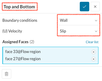
Set the Slip Wall boundary condition.

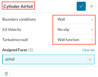
Set the Wall boundary condition to the Cylinder Airfoil.

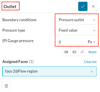
Set the Outlet boundary condition.

Advanced Concepts

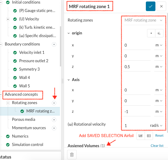
Click on Advanced Concepts, and add MRF Rotating Zones by clicking +
MRF Rotating Zone characteristics must be set as given here, by selecting the saved selection Airfoil as the Assigned Volume.

Numerics and Simulation Control

Set the ‘Numerics’ as given in the ‘FINISHED PROJECT’.

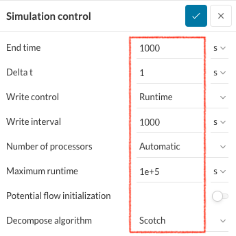
Input the following values under the ‘Simulation Control’.

Result Control

In the ‘Result Control’ section, select + next to ‘Force and Moments’
To calculate the ‘Forces and Moments’, enter the values as given in the snippets, and select the Cylindrical Airfoil from the SAVED SELECTION.
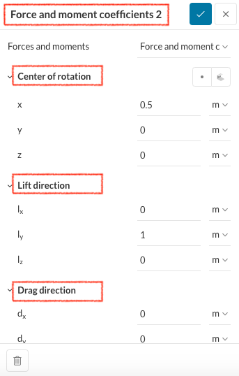
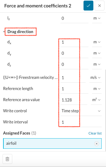
To calculate the ‘Force and Moment Coefficients’, enter the values as given in the snippets below, and select the Cylindrical Airfoil from the SAVED SELECTION.

Mesh Generation

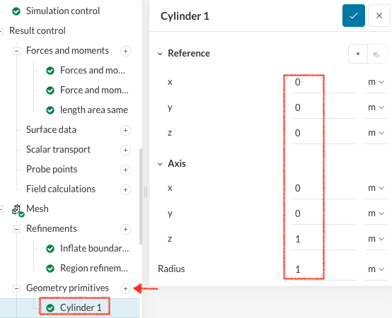
Below the Mesh Settings, click ‘+’ next to Geometry Primitives, and create the following geometry primitives, which would be used in creating the region refinements in the next step for meshing.

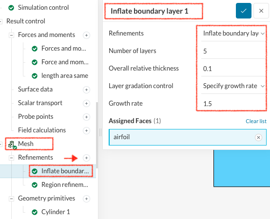
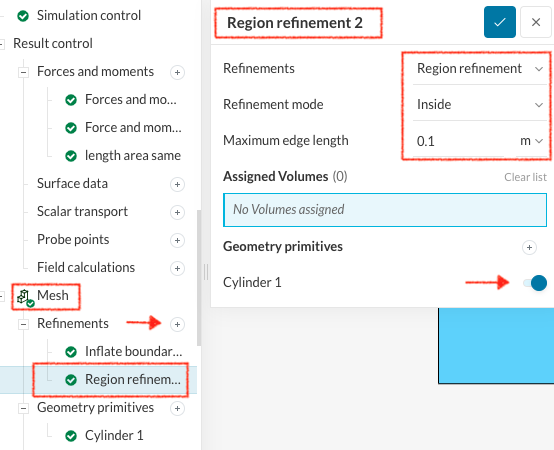
Geometry Primitive Cylinder 2 Creation Set Up

Click on Mesh, and Click ‘+’ next to Refinements, and add the following Inflate Boundary Layer & Region refinement for the cylinder as given below.

Now after creating the geometry primitives, and adding the suitable region refinements for creating fine mesh, let’s set up the mesh characteristics.

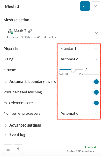
Click on Mesh, and make changes to the Mesh Settings.
Following the above, Click Generate to generate Mesh, and wait for the mesh to get generated.

NOTE: Check the Event Log below the dialogue box once the mesh is generated to check for the mesh quality before proceeding. If the mesh is not correctly generated, Simulation Run in the next stage can get terminated prematurely.

Simulation

To initiate the simulation, follow these steps:

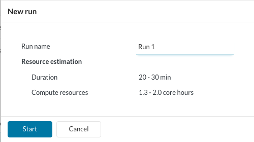
Expand the ‘Simulation Runs’ section by clicking on the ‘+‘ symbol.
Then, select the ‘Run‘ option, and click Start to start the simulation process. This action will prompt the software to execute the simulation based on the defined parameters and settings.

Processing

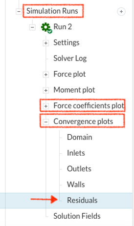
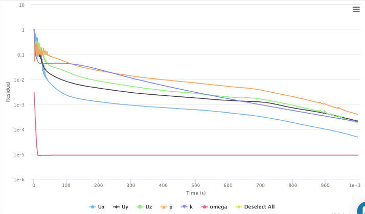
Select the ‘Convergence plots’ below ‘Run’ to check for convergence. In an iterative method, residuals represent the disparities in the solution. Achieving numerical precision involves minimizing these residuals.

Typically, aiming for residuals below 1e-3 is a suitable threshold to proceed to the next assessment.

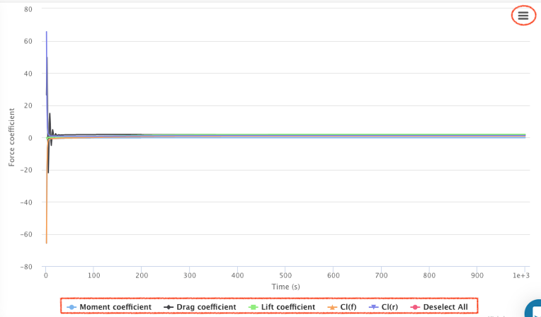
Another aspect to consider is examining the exact values for Force coefficients, such as the coefficient of drag, lift, moment, and so forth, to ascertain their convergence.

This entails analyzing whether these coefficients have stabilized and reached consistent values over successive iterations, indicating convergence in the solution.

Post- Processing

Once the simulation is ‘Complete‘, you can access the post-processing environment by clicking on ‘Solution Fields’ or ‘Post-process results’.

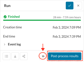
After checking the residuals, if you think it has not yet been converged, you will see the “Continue to run >>” icon, in which you can enter the end time to be your present end time and increase the maximum run time.

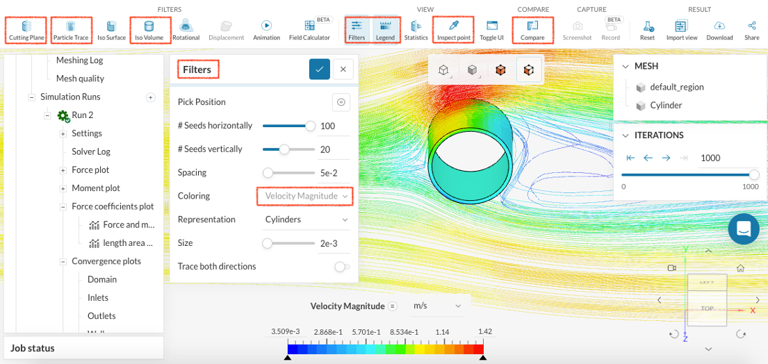
If not, continue by selecting ‘Post-process results.’ See below for all available post-processing options in SimScale:

Cut Plane: Slice the domain to visualize parameters on the plane.
Vectors: Plot vector fields to represent quantities like velocity or force.
Contour Plot: Display scalar field data using contour lines.
Probe Points: Insert points to extract data at specific locations.
Particle Trace: Generate streamlines from seed faces to observe flow patterns.
Iso Surface: Highlight regions with specific scalar values.
Iso Volume: Highlight regions within a defined scalar value range.
Rotational View: Inspect rotational regions by creating blade-to-blade views.
Animation: Create animations of simulation results.
Field Calculator: Generate new fields using predefined functions and operators.
Compare: Visualize result fields from two different simulations side by side.

Please refer to the accompanying image to explore the full range of available options for post-processing. These options provide diverse tools for analyzing and visualizing simulation results in SimScale.

Repeat

Follow the steps outlined above for other Reynolds numbers, while adjusting the velocity values, and relevant numerical parameters as specified in the following tables provided. For a clearer understanding, you can refer to the completed project.

Incoming Flow Velocity(m/s)	Spinning velocity(rad/s)
2	1
1	1
0.564	1

VIEW THE FINISHED PROJECT

VALIDATION RESULTS

GET STARTED WITH YOUR OWN PROJECT