Laminar Flow Analysis in a Pipe
MODULE
AIM
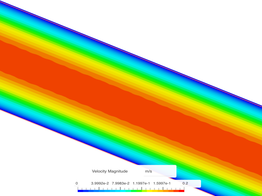
To investigate the pressure drop and visualize the velocity profile in laminar flow through a pipe.
QUICK PEEK INTO THE TEXTBOOK
Review the TEXTBOOK to refresh your understanding of basic concepts before advancing to more complex material.
SimScale Tutorial: Laminar Flow in a Pipe
This tutorial aims to investigate the pressure drop and visualize the velocity profile in laminar flow through a pipe.
Flow Simulation Set Up
Dimensions
A cylindrical pipe with a diameter of 0.01 𝑚, and a length of 10 𝑚.
Analysis Type
Incompressible steady-state analysis.
Turbulence Model
Laminar flow
Mesh and Element Types
Three structured hexahedral meshes generated using the hex-dominant automatic algorithm, refined with a growth rate of 1.25.
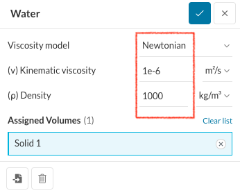
Fluid : Water
Initial Conditions:
- (𝜈) Kinematic viscosity = 10-6 𝑚2/𝑠
Velocity Profile Definition
The parabolic velocity profile through a circular pipe in a laminar flow is approximated as follows:
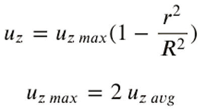
where 𝑢𝑧 is the z-component of the velocity along the axis, 𝑢𝑧𝑎𝑣𝑔 is the average inlet velocity, 𝑢𝑧𝑚𝑎𝑥 is the maximum velocity that occurs at the centerline, 𝑟 is the radial distance from the centerline, and 𝑅 is the radius of the circular pipe.
Boundary Conditions
The following boundary conditions are applied to the corresponding pipe surfaces:
| Face | Boundary type | Value |
| Inlet | Velocity inlet | Fixed value of 2×0.1×(1−(((𝑥)2+(𝑧)2)0.5/0.005)2) 𝑚/𝑠 in the y-direction |
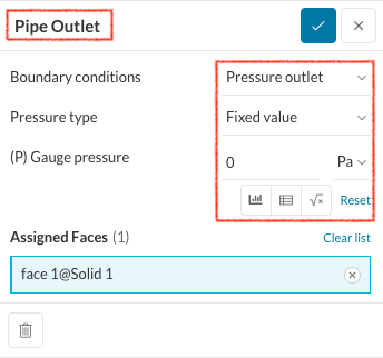
| Outlet | Pressure outlet | Fixed value of 0 𝑃𝑎 |
| Pipe Surface | Wall | No-slip |
Let’s now delve into the SimScale process one step at a time for this particular problem.
Just a heads-up: The ideal way to begin is by creating a ‘New Project‘ and then importing the CAD model. However, we’ve already taken care of the steps for you, including importing the CAD model. You can get started right away with the ‘Create Simulation‘ step.
Prepare the CAD Model and Select the Analysis Type
Open a ‘New Project’ & import the CAD model
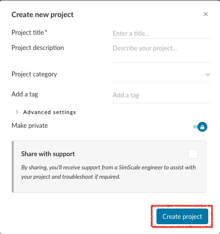
- Click open the new project, and fill the details as following dialogue box appears.
- Once details are entered, Click ‘Create Project‘.
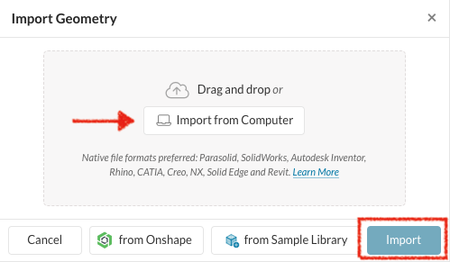
- Click + next to GEOMETRIES, and import the CAD model
Create Simulation
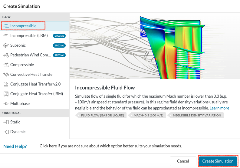
- Select ‘Incompressible’ and click Create Simulation
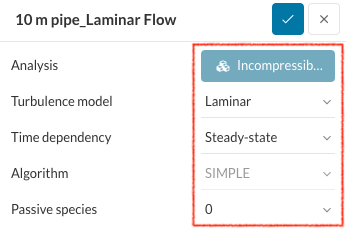
- Once the Simulation has been created, you can rename it, and choose ‘Laminar‘ to be the Turbulence model and edit the other characteristics as shown here.
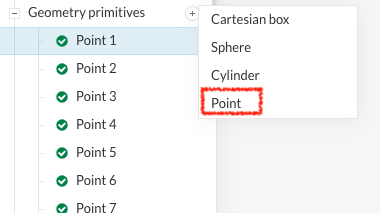
- Click ‘+’ next to Geometry Primitives
- Add points as per the given coordinates as in the finished project file, by selecting ‘Point’ from the drop down menu.
Assigning the Material and Boundary Conditions
Define a Material
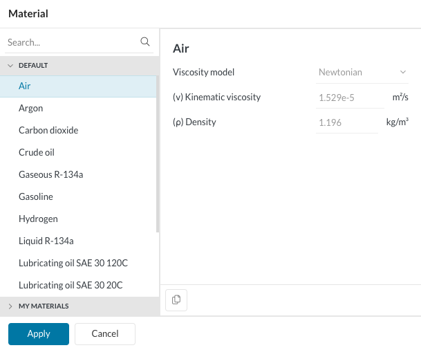
- Select ‘Air’ by clicking ‘+’ next to ‘Material’.
- Edit the values of the default coefficients to the set values as given in the image.
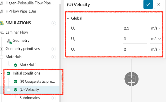
Define the Initial Conditions
- Set the Initial Conditions, namely (P) Gauge static pressure to be ‘0 Pa’, and set the (U) Velocity(Global) to be as given here.
Define Boundary Conditions
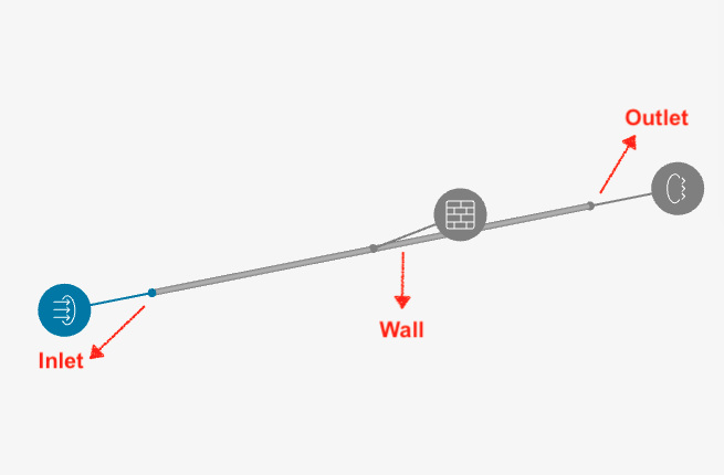
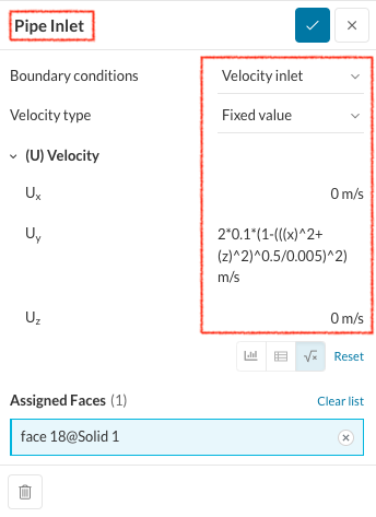
- Set the Inlet boundary condition.
- Set the Outlet boundary condition.
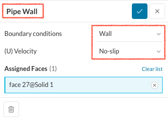
- Set the Wall boundary condition.
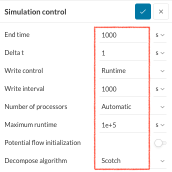
Simulation Control
- Set the ‘Numerics’ as given in the ‘FINISHED PROJECT’.
- Input the following values under the ‘Simulation Control’.
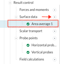
Result Control
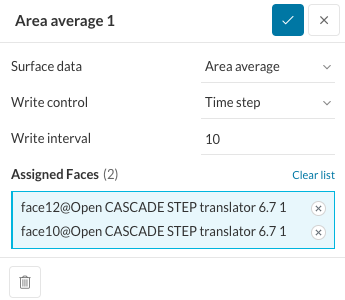
- Now, it’s time to set up the ‘Area Average‘.
- Below ‘Result Control’, click ‘+’ next to Surface Data, and enter the following values.
- To calculate area averages and other parameters like velocity components at each probe point and record them, it’s crucial to choose the suitable probe points.
- For example, consider creating a set of points named ‘Probe Points along the Length’. Click ‘Probe Points’ and turn on the points appropriate set of points to be added to the list, and name them as ‘Probe Points along the Length’.
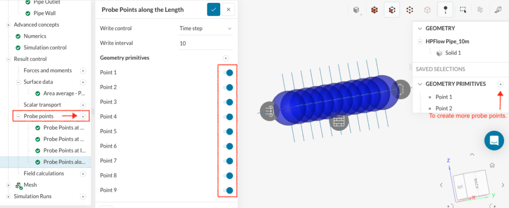
- Do the same for other sets.
NOTE: Please note that the example provided is just a demonstration. Refer to the Finished Project for the specific number of lists and corresponding probe points. Feel free to create your own lists tailored to your preferences. The rationale behind these selections will be explained at the end of this module.
Mesh Generation
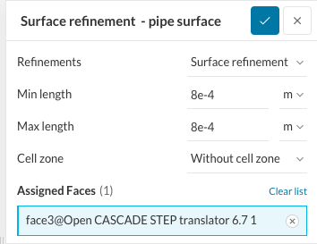
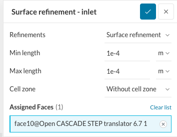
- Click on Mesh, and Click ‘+’ next to Surface Refinement, and add the following surface refinement for the inlet, and pipe surface as given below.
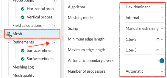
- Following which, click on Mesh, and make changes to the Mesh Settings as given.
Following the above, Click Generate to generate Mesh, and wait for the mesh to get generated.
NOTE: Check the Event Log below the dialogue box once the mesh is generated to check for the mesh quality before proceeding. If the mesh is not correctly generated, Simulation Run in the next stage can get terminated prematurely.
Simulation
To initiate the simulation, follow these steps:
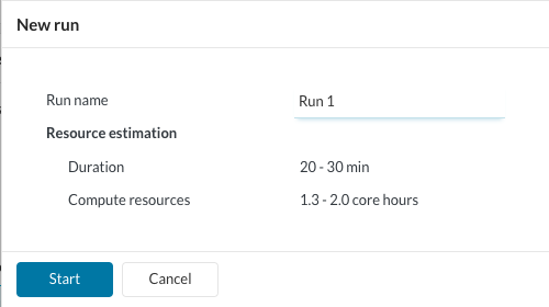
- Expand the ‘Simulation Runs’ section by clicking on the ‘+‘ symbol.
- Then, select the ‘Run’ option to start the simulation process. This action will prompt the software to execute the simulation based on the defined parameters and settings.
Post- Processing
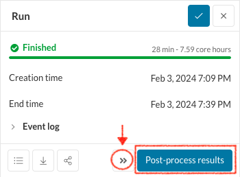
- Once the simulation is ‘Complete‘, you can access the post-processing environment by clicking on ‘Solution Fields’ or ‘Post-process results’.
After checking the residuals, if you think it has not yet been converged, you will see the “Continue to run >>” icon, in which you can enter the end time to be your present end time and increase the maximum run time.
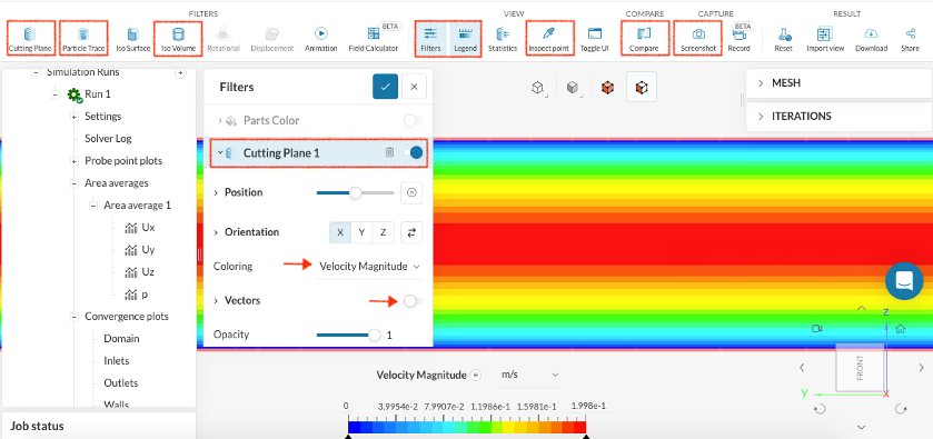
If not, continue by selecting ‘Post-process results.’ See below for all available post-processing options in SimScale:
- Cut Plane: Slice the domain to visualize parameters on the plane.
- Vectors: Plot vector fields to represent quantities like velocity or force.
- Contour Plot: Display scalar field data using contour lines.
- Probe Points: Insert points to extract data at specific locations.
- Particle Trace: Generate streamlines from seed faces to observe flow patterns.
- Iso Surface: Highlight regions with specific scalar values.
- Iso Volume: Highlight regions within a defined scalar value range.
- Rotational View: Inspect rotational regions by creating blade-to-blade views.
- Animation: Create animations of simulation results.
- Field Calculator: Generate new fields using predefined functions and operators.
- Compare: Visualize result fields from two different simulations side by side.
Please refer to the accompanying image to explore the full range of available options for post-processing. These options provide diverse tools for analyzing and visualizing simulation results in SimScale.
Pressure Drop
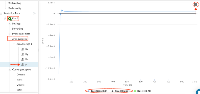
- Navigate to the ‘Simulation Run’ section.
- Click on ‘Area Averages’.
- Select ‘p’ to display the plot showing pressure values for both the inlet and outlet faces of the pipe across each iteration.
- Option 1: Click on the dropdown icon at the top-right corner to download the .csv file. Download the CSV file and observe the converged ‘p‘ values corresponding to the end time.
- Option 2: Alternatively, check the final value directly from the live plot at the end time.
Velocity Profile
The values of velocity components at various probe points, including those along the radial and axial directions of the pipe.
- Choose the ‘Probe Point plots‘ located below ‘Simulation Run’.
- Click on the dropdown icon at the top-right corner to download the .csv file.
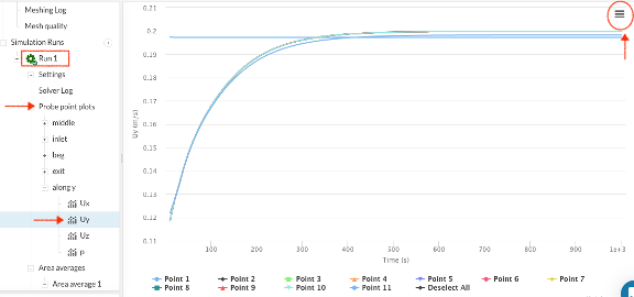
- The downloaded file contains precise velocity values for each probe point and iteration until the ‘end time‘.
- Utilize MATLAB/Python/any programming language you’re familiar with to plot the velocity profile using the data from the downloaded .csv files.